The Global Urban Demographic Dataset (GUDD), version 1 provides a comprehensive overview of demographic changes in urban areas worldwide. This analysis focuses on the key trends observed in Gudd, highlighting shifts in population size, age distribution, and migration patterns over the past two decades.
In this tutorial, we will explore demographic changes in dependency ratios–including youg and old dependency ratios– male-female ratios in young, working and elderly populations, and their implications for urban planning and policy-making. We will also examine how age-sex pyramid structures have evolved in Gudd, providing insights into the changing needs of the population.
We will use Python to analyze the data, leveraging libraries such as pandas for data manipulation and matplotlib for visualization. The analysis will include:
Downloading and working with the GUDD dataset
Using geoparquet static boundaries to determine temporal changes in demographic characteristics
Visualizing changes in age-sex pyramids and dependency ratios
Interpreting the results to inform urban planning and policy decisions
Downloading the GUDD Dataset
THe GUDD dataset was developed by Andrew Zimmer, Nina Brooks, Andrea E. Gaughan & Cascade Tuholske. Their work can be cited as follows:
Zimmer, A., Brooks, N., Gaughan, A.E. et al. Global divergence in urban demographic change and migration patterns. Nat Cities 3, 599–607 (2026). https://doi.org/10.1038/s44284-026-00447-7
The GUDD dataset is available for download from the Harvard Dataverse. You can access the dataset using the following link: GUDD Dataset.
We will use the gudd_static_boundaries_lookup.geoparquet file as a reference for the static boundaries of Gudd, which will help us analyze demographic changes over time. Using the static boundaries, we can control for spatial variations and focus on temporal changes in demographic characteristics.
The geoparquet file contains the spatial geometries of the static boundaries, as well as a year field and an ID field that can be used to link the boundaries to the demographic data. Since the boudnaries are static, the year field will be the same for all records, but it is important to note that the demographic data may vary over time. We will use the ID field to link the static boundaries to the demographic data in the GUDD dataset.
Download the CSV file gudd_all_static_boundaries.csv that contains raw population counts for each age-sex cohort, derived using static boundaries. The CSV file is also available from the Harvard Dataverse.
Working with the GUDD Dataset
First, we will load the GUDD CSV file into a pandas DataFrame. We will then explore the dataset to understand its structure and contents. The GUDD dataset contains information about population counts for different age-sex cohorts, which will be used to analyze demographic changes over time.
Building the Age-Sex Pyramids for a country of interest
We can start by working with the GUDD all static boundaries CSV, which provides 5-year age groups and sex-specific population data. This data will be used to create age-sex pyramids that visualize the demographic structure of the population over time.
Let’s load the GUDD CSV file into a pandas DataFrame and preview the table columns and head. We will also check for any missing values in the dataset.
import pandas as pd# define the path to the GUDD CSV filegudd_all_csv_path =r"D:\jmartine\user_guides\gudd\gudd_all_static_boundaries.csv"# load the GUDD CSV file into a pandas DataFramegudd_all_data = pd.read_csv(gudd_all_csv_path)# preview the table columns and headprint(gudd_all_data.columns)
According to the GUDD readme file, the dataset contains columns for irregular age groups for Ages <1 and 1-4. All other age groups are in 5-year intervals, up to 80+. The dataset also includes columns for sex-specific population counts, as well as total population counts for each age group.
We can combine the irregular age groups into a single age group of 0-4, and then create a new column for the 5-year age groups. This will allow us to create age-sex pyramids that are consistent across all age groups.
## add a new column that sums f_00 and f_01, and m_00 and m_01, to create a new age group of 0-4gudd_all_data['f_0_4'] = gudd_all_data['f_00'] + gudd_all_data['f_01']gudd_all_data['m_0_4'] = gudd_all_data['m_00'] + gudd_all_data['m_01']
Now that our data is prepared we can create a function to generate age-sex pyramids by inputting the country and years of interest as required parameters.
These visualizations will help us understand how the population structure has changed over time, providing insights into demographic trends and potential implications for urban planning and policy-making.
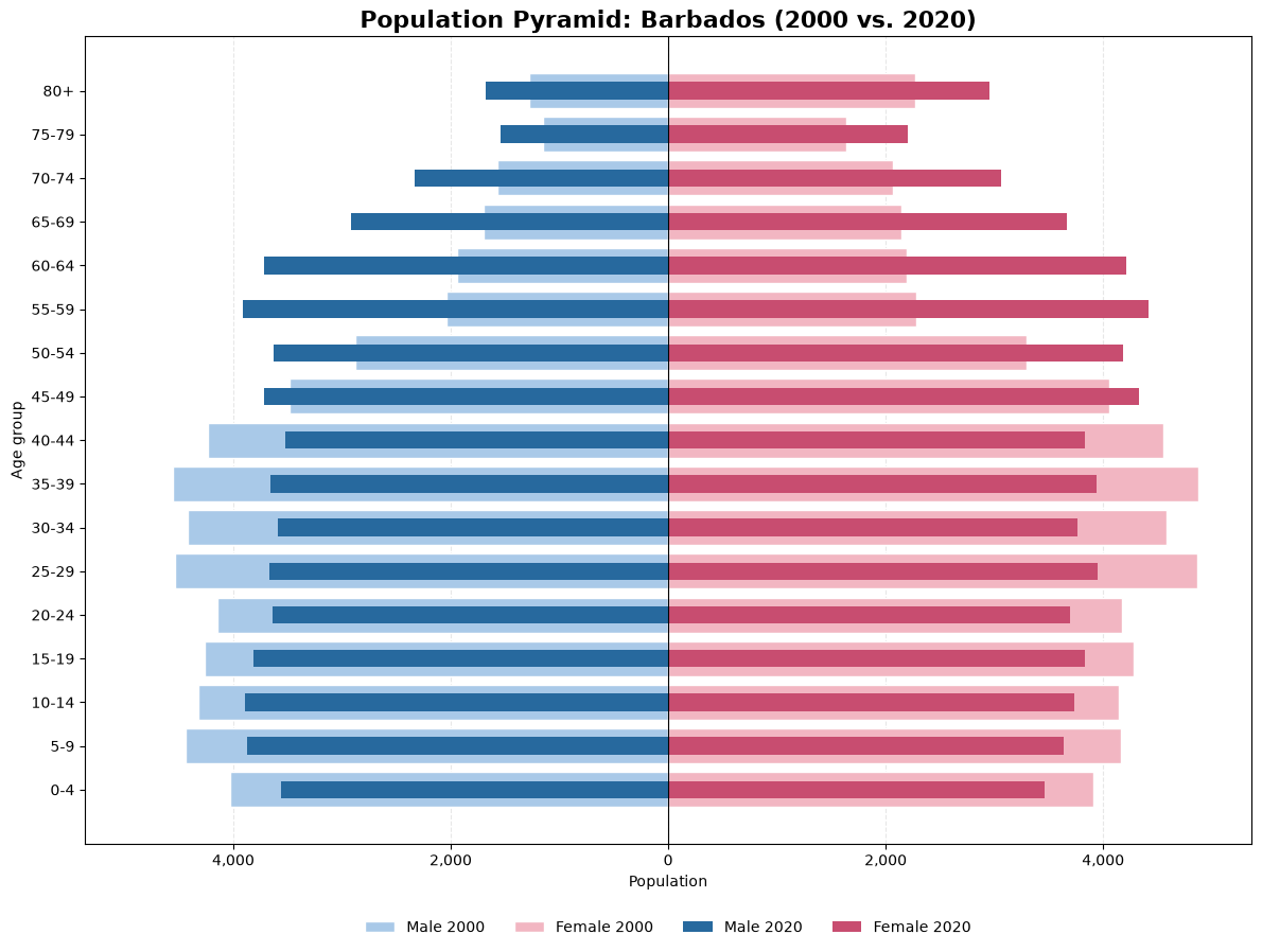
To visualize the age-sex pyramids, we will use the matplotlib and numpy libraries to create bar charts that represent the population counts for each age-sex cohort. The x-axis will represent the population counts, while the y-axis will represent the age groups. We will create separate bars for males and females, allowing us to compare the population distribution between the two sexes.
import matplotlib.pyplot as pltimport numpy as np## select columns of interest for age-sex cohortsf_age_sex_columns = ['f_0_4', 'f_05', 'f_10', 'f_15', 'f_20', 'f_25', 'f_30', 'f_35', 'f_40', 'f_45', 'f_50', 'f_55', 'f_60', 'f_65', 'f_70', 'f_75', 'f_80']m_age_sex_columns = ['m_0_4', 'm_05', 'm_10', 'm_15', 'm_20', 'm_25', 'm_30', 'm_35', 'm_40', 'm_45', 'm_50', 'm_55', 'm_60', 'm_65', 'm_70', 'm_75', 'm_80']# Age group labelsage_groups = ['0-4', '5-9', '10-14', '15-19', '20-24','25-29', '30-34', '35-39', '40-44', '45-49','50-54', '55-59', '60-64', '65-69', '70-74','75-79', '80+']def plot_population_pyramid(df, country, year1=2000, year2=2020):# Filter country country_df = df[df['Country'] == country]# Get observations for each year data1 = country_df[country_df['year'] == year1] data2 = country_df[country_df['year'] == year2]if data1.empty or data2.empty:raiseValueError(f"Missing data for {country} in {year1} or {year2}" )# Extract population values# Assumes one row per country/year data1 = data1.iloc[0] data2 = data2.iloc[0] m1 = data1[m_age_sex_columns].to_numpy(dtype=float)[::-1] f1 = data1[f_age_sex_columns].to_numpy(dtype=float)[::-1] m2 = data2[m_age_sex_columns].to_numpy(dtype=float)[::-1] f2 = data2[f_age_sex_columns].to_numpy(dtype=float)[::-1]# Reverse age labels age_labels = age_groups[::-1] y = np.arange(len(age_labels))# Create figure fig, ax = plt.subplots(figsize=(12, 9))# Year 1 - lighter colors ax.barh( y, -m1, color='#A9C9E8', label=f'Male {year1}', height=0.8, edgecolor='white' ) ax.barh( y, f1, color='#F2B6C2', label=f'Female {year1}', height=0.8, edgecolor='white' )# Year 2 - darker colors ax.barh( y, -m2, color='#27699E', label=f'Male {year2}', height=0.4 ) ax.barh( y, f2, color='#C84D70', label=f'Female {year2}', height=0.4 )# Center line ax.axvline(0, color='black', linewidth=0.8)# Labels ax.set_yticks(y) ax.set_yticklabels(age_labels) ax.set_ylabel('Age group') ax.set_xlabel('Population')# Symmetric horizontal scale max_population = np.nanmax([m1, f1, m2, f2]) ax.set_xlim(-max_population *1.1, max_population *1.1 ) ax.xaxis.set_major_formatter( plt.FuncFormatter(lambda x, _: f'{abs(x):,.0f}') ) ax.set_title(f'Population Pyramid: {country} ({year1} vs. {year2})', fontsize=16, fontweight='bold' ) ax.grid(axis='x', linestyle='--', alpha=0.3) ax.set_axisbelow(True) ax.legend( loc='lower center', bbox_to_anchor=(0.5, -0.13), ncol=4, frameon=False ) ax.invert_yaxis() plt.tight_layout() plt.show()
Now we can use this function to create age-sex pyramids for the years 2000 and 2020 allowing us to select a country of interest. The function will take the DataFrame, country name, and years as input parameters, and will generate the age-sex pyramids for the specified years.
What are some of the changes in the age-sex pyramids for the country of interest between 2000 and 2020? How do these changes reflect broader demographic trends in the country, and what implications might they have for urban planning and policy-making?
Demographic Changes in GUDD Dataset from 2000 to 2020
We can start by working with the GUDD tabular data that contains demographic changes between 2000 and 2020. The CSV file gudd_change_2000_2020_static_boundaries.csv is used to analyze the changes in population counts for each age-sex cohort over the two decades. We will load this CSV file into a pandas DataFrame and preview its columns and head to understand its structure.
# define the path to the GUDD CSV filegudd_change_csv_path =r"D:\jmartine\user_guides\gudd\gudd_change_2000_2020_static_boundaries.csv"# load the GUDD CSV file into a pandas DataFramegudd_change_data = pd.read_csv(gudd_change_csv_path)# preview the table columns and headprint(gudd_change_data.columns)
With this information, we can analyze changes in dependency ratios, male-female ratios, and other demographic characteristics over the two decades. This analysis will provide insights into the changing needs of the population and inform urban planning and policy decisions.
Lets first determine on average how dependency ratios for total, young and old populations have changed between 2000 and 2020 over each continent.
# Dependency ratio change columnsdependency_columns = ['total_dr_Delta','young_dr_Delta','old_dr_Delta']# Calculate mean change by continentcontinent_changes = ( gudd_change_data .groupby('Continent')[dependency_columns] .mean() .round(3))# sort by total_dr_Delta in descending ordercontinent_changes = continent_changes.sort_values(by='total_dr_Delta', ascending=False)print(continent_changes)
                                  total_dr_Delta  young_dr_Delta  old_dr_Delta
Continent
Europe                                     0.061          -0.011         0.072
Australia and New Zealand                  0.047          -0.018         0.065
Northern America                           0.029          -0.040         0.069
Eastern and South-Eastern Asia            -0.049          -0.118         0.068
Sub-Saharan Africa                        -0.069          -0.072         0.003
Oceania                                   -0.100          -0.123         0.024
Northern Africa and Western Asia          -0.121          -0.137         0.016
Latin America and the Caribbean           -0.131          -0.170         0.039
Central and Southern Asia                 -0.157          -0.178         0.022
What can the changing dependency ratios tell us about the demographic trends in each continent, and how might these trends impact urban planning and policy-making in the future?
Changes in sex ratios by continent
Similarly, we can analyze changes in sex ratios for total, young, working and elderly populations over the two decades.
# sex ratio change columnssex_ratio_columns = ['young_sr_Delta', 'working_sr_Delta', 'old_sr_Delta', 'total_sr_Delta',]# Calculate mean change by continentcontinent_changes_sr = ( gudd_change_data .groupby('Continent')[sex_ratio_columns] .mean() .round(3))# sort by total_sr_Delta in descending ordercontinent_changes_sr = continent_changes_sr.sort_values(by='total_sr_Delta', ascending=False)print(continent_changes_sr)
                                  young_sr_Delta  working_sr_Delta  \
Continent
Northern Africa and Western Asia           0.001             0.016
Central and Southern Asia                  0.012             0.007
Oceania                                    0.002             0.003
Sub-Saharan Africa                        -0.004            -0.005
Australia and New Zealand                 -0.002            -0.002
Europe                                     0.003            -0.006
Latin America and the Caribbean           -0.002            -0.002
Northern America                          -0.000            -0.004
Eastern and South-Eastern Asia             0.002             0.003

                                  old_sr_Delta  total_sr_Delta
Continent
Northern Africa and Western Asia         0.000           0.015
Central and Southern Asia               -0.024           0.001
Oceania                                 -0.004          -0.003
Sub-Saharan Africa                      -0.052          -0.007
Australia and New Zealand                0.006          -0.008
Europe                                   0.052          -0.008
Latin America and the Caribbean         -0.004          -0.011
Northern America                         0.019          -0.011
Eastern and South-Eastern Asia          -0.014          -0.013
What can the changing sex ratios tell us about the demographic trends in each continent, and how might these trends impact urban planning and policy-making in the future?
Visualizing Demographic Changes
To open a geoparquet file in Python, we can use the geopandas library. First, we need to install the library if it is not already installed. We also define the path to the gudd_static_boundaries_lookup.geoparquet file, which contains the static boundaries for Gudd:
import geopandas as gpd#define the path to the static boundaries fileboundaries_path =r"D:\jmartine\user_guides\gudd\gudd_static_boundaries_lookup.geoparquet"# open the geoparquet file using geopandasgudd_boundaries = gpd.read_parquet(boundaries_path)
Once we have loaded the static boundaries, we can explore the dataset to understand its structure and contents. The gudd_boundaries GeoDataFrame contains information about the geographic boundaries of Gudd, which will be used to analyze demographic changes over time.
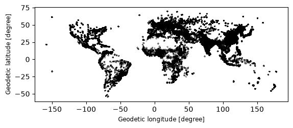
Let’s start with visualizing the static boundaries of Gudd to get a better understanding of the area we are analyzing. We can use the plot method from matplotlib and geopandas to create a simple map of the static boundaries.
# Visualize the static boundaries of Gudd with a thick border linegudd_boundaries.plot(edgecolor='black', linewidth=2)
Now we can view the tabular data of the static boundaries to see the attributes associated with each boundary. This will help us understand the demographic characteristics of Gudd and how they have changed over time.
#view the column names of the static boundariesprint(gudd_boundaries.columns)# view the tabular data of the static boundariesprint(gudd_boundaries.head())
With the ID_UC_G0 column, we can link the static boundaries to the demographic data in the GUDD dataset. This will allow us to analyze changes in population counts for each age-sex cohort over time, providing insights into demographic trends and potential implications for urban planning and policy-making.
Visualizing changes in dependency ratios and sex ratios
We can use the tabular data of demographic changes to visualize changes in dependency ratios and sex ratios over the two decades. This will help us understand how the population structure has evolved and what implications it may have for urban planning and policy-making.
First, we append both tables to the geopandas dataframe of static boundaries, allowing us to visualize the changes in dependency ratios and sex ratios on a map. We can use the plot method from matplotlib and geopandas to create maps that show the changes in dependency ratios and sex ratios for each continent.
## join the static boundaries with the dependency ratio changes by city using the ID_UC_G0 column as the keygudd_boundaries_with_changes = gudd_boundaries.merge( gudd_change_data, on='ID_UC_G0', how='left')gudd_boundaries_with_changes.columns
Now that we have joined the static boundaries with the demographic changes, we can create visualizations to show how dependency ratios and sex ratios have changed over time. This will help us understand the demographic trends in each continent and inform urban planning and policy-making decisions.
Since this is a global dataset, it would be difficut to visualize the polygons of each city, so we first use the cities centroids to visualizr the changes in demographic characteristics. We can calculate the centroids of the static boundaries using the centroid attribute of the GeoDataFrame, and then create a new GeoDataFrame containing the centroids and the demographic changes.
# Calculate city centroidsgudd_centroids = gudd_boundaries_with_changes.copy()gudd_centroids['geometry'] = gudd_centroids.geometry.centroid
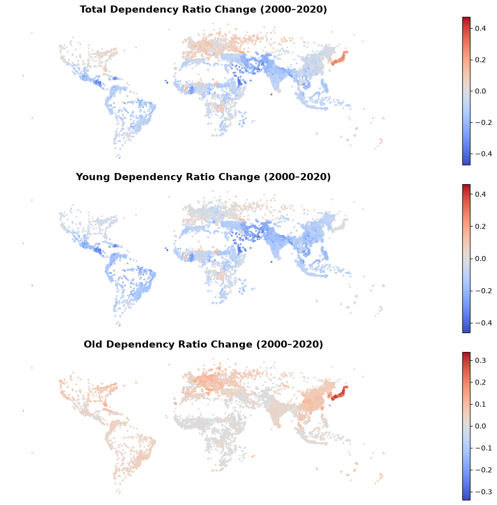
# plot the static boundaries with the dependency ratio changes import matplotlib.pyplot as pltfrom matplotlib.colors import TwoSlopeNorm# Variables to plotvariables = ['total_dr_Delta','young_dr_Delta', 'old_dr_Delta']# Map titlestitles = ['Total Dependency Ratio Change (2000–2020)','Young Dependency Ratio Change (2000–2020)','Old Dependency Ratio Change (2000–2020)', ]# Create 2x2 subplot layoutfig, axes = plt.subplots(3,1, figsize=(24, 10))# Plot each variablefor variable, title, ax inzip(variables, titles, axes.flatten()):# Calculate symmetric color scale max_abs = gudd_centroids[variable].abs().max()# Plot centroids gudd_centroids.plot( column=variable, cmap='coolwarm', norm=TwoSlopeNorm(vmin=-max_abs, vcenter=0, vmax=max_abs), markersize=3, legend=True, ax=ax, alpha=0.8 ) ax.set_title(title, fontsize=14, fontweight='bold') ax.set_axis_off()plt.tight_layout()plt.show()
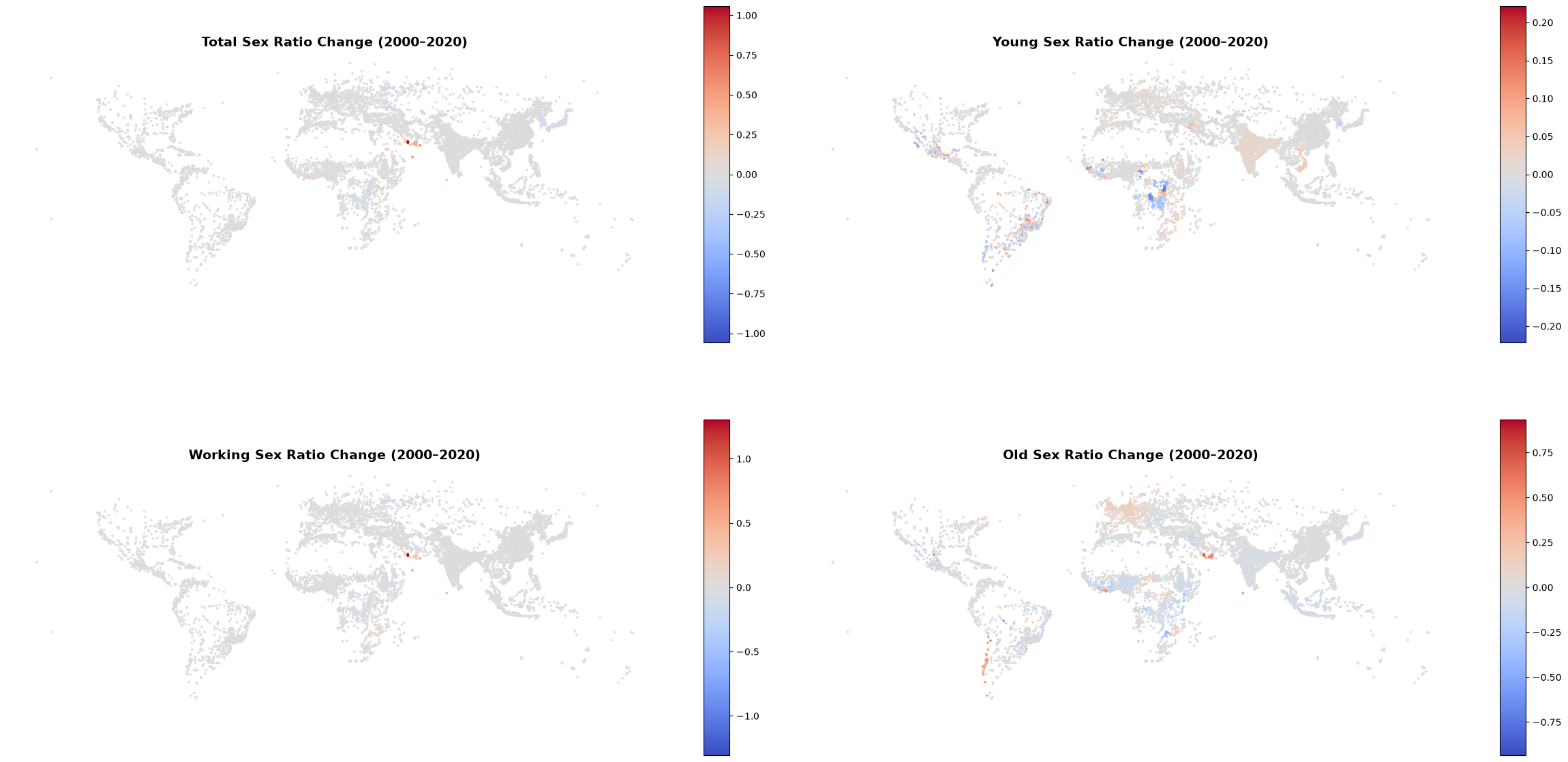
# plot the static boundaries with the sex ratio changes# Variables to plotvariables = ['total_sr_Delta','young_sr_Delta','working_sr_Delta','old_sr_Delta']# Map titlestitles = ['Total Sex Ratio Change (2000–2020)','Young Sex Ratio Change (2000–2020)','Working Sex Ratio Change (2000–2020)','Old Sex Ratio Change (2000–2020)']# Create 2x2 subplot layoutfig, axes = plt.subplots(2, 2, figsize=(24, 14))# Plot each variablefor variable, title, ax inzip(variables, titles, axes.flatten()):# Calculate symmetric color scale max_abs = gudd_centroids[variable].abs().max()# Plot centroids gudd_centroids.plot( column=variable, cmap='coolwarm', norm=TwoSlopeNorm(vmin=-max_abs, vcenter=0, vmax=max_abs), markersize=3, legend=True, ax=ax, alpha=0.8 ) ax.set_title(title, fontsize=14, fontweight='bold') ax.set_axis_off()plt.tight_layout()plt.show()
What do the visualizations of changes in dependency ratios and sex ratios tell us about the demographic trends in cities around the world, and how might these trends impact urban planning and policy-making in the future?
Conclusion and Discussion
Using the GUDD dataset, we have analyzed demographic changes in urban areas worldwide between 2000 and 2020. By examining changes in dependency ratios, sex ratios, and age-sex pyramids, we have gained insights into the evolving population structure and its implications for urban planning and policy-making at a global scale.
This dataset provides a valuable resource for researchers, policymakers, and urban planners to understand demographic trends and make informed decisions that address the needs of the population.
For more information on the GUDD dataset, please refer to the original publication by Zimmer et al. (2026) and the Harvard Dataverse repository where the dataset is hosted.
This tutorial was produced by CIESIN at Columbia University, 2026.
All materials used and produced by CIESIN are licensed under a Creative Commons Attribution 4.0 International License (CC BY 4.0).