Nigeria_Settlement_Block_GreenSpace_Analysis

Author: Matthew Walter

Settlement Extents v4 are geographic data products that have been produced by CIESIN and GRID3 for both Nigeria and the Democratic Republic of the Congo. The major innovation over v3 is the inclusion of Settlement Blocks, which represent small homogeneous spatial units split by linear features such as roads and rivers. Blocks include a number of block-level variables to describe urban morphology, including building characteristics, settlement characteristics, and green space.

This notebook demonstrates how to import Settlement Extents v4 and utilize their spatial information by attempting to answer the following question from the perspective of an urban planner:

What areas of Lagos should be targeted for urban greening given limited resources to have the largest impact?

To answer this question we identify blocks that are: 1. Likely residential 2. Likely to contain the most residents 3. Contain the least green space

The Settlement Extent Blocks contain a variety of variables including block-level building characteristics, extent type, building height, vegetation indices, and classifications based on building characteristics. All of the block-level variables are described in the table below.

Block, Settlement Extent, Building, Classification, and Remote-Sensing Variables

Field Name	Description
Block Characteristics	Block-level geographic and building characteristics.
`block_id`	Unique identifier for each block.
`country`	Country name.
`iso3`	Three-letter ISO country code.
`block_area_sqm`	Block area in square meters.
`block_perimeter`	Block perimeter in meters.
`block_neighbor_count`	Number of neighboring blocks.
`building_count`	Total count of buildings, taken at the center point, within the block.
`building_area_min`	Area of the smallest building whose centroid falls within the block, measured in square meters.
`building_area_max`	Area of the largest building whose centroid falls within the block, measured in square meters.
`building_area_sum`	Sum of building area values within the block, measured in square meters. Unlike building count and the minimum, maximum, median, and standard deviation metrics, this field is calculated using the building area contained within the block rather than buildings whose centroids fall within the block.
`building_area_median`	Median building footprint area for buildings whose centroids fall within the block, measured in square meters.
`building_area_stdev`	Standard deviation of building footprint area for buildings whose centroids fall within the block, measured in square meters.
`building_area_percentage`	Sum of building area values within the block, as described in `building_area_sum`, divided by the block area and expressed as a percentage.
`building_count_density`	Building count, taken at the center point, divided by block area, expressed per hectare.
`building_count_density_quantile_rank`	Quantile rank of building count density across all blocks.
`building_area_sum_quantile_rank`	Quantile rank of total building area across all blocks.
Settlement Extent	Variables describing the original settlement extent associated with each block.
`extent_type`	Categorical settlement classification for the block: Built-up Area (BUA), Small Settlement Area (SSA), or Hamlet.
`mgrs_code`	Military Grid Reference System (MGRS) code of the settlement for which the block belongs.
`blocks_per_settl_extent`	Number of blocks within the extent of the settled area based on `mgrs_code`.
Google 2.5D Building Footprints	Building height summaries derived from Google Open Buildings 2.5D data.
`gbuilding_max_height`	Maximum building height per block, measured in meters, with the temporal maximum taken across 2021–2023.
`gbuilding_mean_height`	Mean building height per block, measured in meters, averaged across 2021–2023.
Remote-Sensing Indices	Remote-sensing indices summarized within each block using cloud-free composites and zonal statistics.
`evi_mean`	Average Enhanced Vegetation Index (EVI) pixel value within a block, calculated from a cloud-free median composite of Sentinel-2 Surface Reflectance imagery collected during 2024.
`ndvi_mean`	Average Normalized Difference Vegetation Index (NDVI) pixel value within a block, calculated from a cloud-free median composite of Sentinel-2 Surface Reflectance imagery collected during 2024.
Classification Variables	Categorical variables derived from building density and building size characteristics.
`bd_class`	Categorical classification of building count density. Defined as Low when `building_count_density` is ≤ 25 and High when `building_count_density` is > 25.
`ma_class`	Categorical classification of maximum building area, measured in square meters. Defined as Low when `building_area_max` is ≤ 700 m² and High when `building_area_max` is > 700 m².
`composite_class`	Composite classification derived from `bd_class` and `ma_class`, with additional classifications for areas identified as Open Space or Airport.

Building and green space analysis

Install and import libraries

# install arcgis API for accessing data
%%capture --no-display
!pip install arcgis
!pip install contextily

import contextily as cx
from pyproj import Transformer
from arcgis.gis import GIS
from arcgis.features import FeatureLayer
from arcgis.geometry.filters import contains
import json
import arcgis
import matplotlib.pyplot as plt
import matplotlib.colors as mcolors

import pandas as pd
import geopandas as gpd

import zipfile
import os

First, we need to read in the settlement blocks for Nigeria from ArcGIS Online and filter down from millions of blocks throughout the countries to just those in Lagos.

# Import roads layer from ArcGIS REST and clip to bounding box
# Read in service for NGA settlements v4.0
layer_url = "https://services3.arcgis.com/BU6Aadhn6tbBEdyk/arcgis/rest/services/GRID3_NGA_settlement_extents_v4_1/FeatureServer/0"
feature_layer = FeatureLayer(layer_url)

# Set bbox in coordinates
bbox = [3.374863,6.392771,3.476830,6.483568]

# transform CRS
transformer = Transformer.from_crs('4326', '3857', always_xy=True)
xmin, ymin = transformer.transform(bbox[0], bbox[1])
xmax, ymax = transformer.transform(bbox[2], bbox[3])

# Create bounding box
query_extent = {"xmin": xmin, "ymin": ymin, "xmax": xmax, "ymax": ymax, "spatialReference": {"wkid": 3857},}

# Write spatial query
query_filter = contains(query_extent, sr=3857)

# Convert to feature set and subset by bounding box
feat = feature_layer.query(geometry_filter=query_filter)

# Convert to geojson
geojson_data = json.loads(feat.to_geojson)

# Convert to geodataframe
gdf = gpd.GeoDataFrame.from_features(geojson_data['features'], crs="3857")

gdf = gdf.to_crs('4326')

gdf.head()

	geometry	fid	block_id	country	iso3	block_area_sqm	block_perimeter	block_neighbor_count	building_count	building_area_min	...	gbuilding_mean_height	blocks_per_settl_extent	building_count_density_quantile_rank	building_max_area_quantile_rank	building_count_density	bd_class	ma_class	composite_class	Shape__Area	Shape__Length
0	POLYGON ((3.39849 6.44807, 3.39854 6.448, 3.39...	2271313	blk_75224	Nigeria	NGA	20492.454318	584.349263	7	43	6.347303	...	11.945839	8169	0.747112	0.986734	20.983333	low	high	bd_low_ma_high	20890.554199	588.748424
1	POLYGON ((3.38985 6.4286, 3.3898 6.42857, 3.38...	2269779	blk_75086	Nigeria	NGA	41557.714573	1153.059272	5	29	25.141318	...	6.303385	29	0.469059	0.999790	6.978247	low	high	bd_low_ma_high	42362.010590	1163.560647
2	POLYGON ((3.39526 6.45403, 3.39531 6.45403, 3....	2272235	blk_75307	Nigeria	NGA	3946.548713	249.272061	6	10	40.507396	...	5.919763	8169	0.790755	0.890610	25.338595	high	low	bd_high_ma_low	4023.305267	252.333716
3	POLYGON ((3.38572 6.45356, 3.38576 6.45353, 3....	2272023	blk_75288	Nigeria	NGA	9289.630859	501.971218	7	5	28.049438	...	4.488005	8169	0.393623	0.965696	5.382345	low	low	bd_low_ma_low	9470.278763	503.470326
4	POLYGON ((3.38678 6.4528, 3.38683 6.45277, 3.3...	2271923	blk_75279	Nigeria	NGA	66722.971868	1652.990319	12	51	8.833626	...	4.065922	8169	0.494185	0.996199	7.643544	low	high	bd_low_ma_high	68019.926620	1690.264861

5 rows × 30 columns

Before we pull out the high building density blocks, we want to make sure non-residential blocks are filtered out. The composite_class variable has a value “bd_low_ma_high” which are blocks with a low number of buildings, but high maxiumum building area. These often represent industrial areas, and thus will be filtered out from the analysis. Open spaces and airports are also non-residential so they will be filtered out as well.

# Convert the crs of our data to match Google Imagery
gdf = gdf.to_crs(epsg=3857)

# Filter out non-residential calsses
exclude_classes = [
    "bd_low_ma_high",
    "open space",
    "airport"
]

gdf_res = gdf[
    ~gdf["composite_class"].isin(exclude_classes)
]


# Plot data
fig, axes = plt.subplots(1, 2, figsize=(22, 10))


# Map the composite classification

gdf.plot(
    ax=axes[0],
    column="composite_class",
    categorical=True,
    legend=True,
    cmap="Set2",
    edgecolor="none"
)

cx.add_basemap(
    axes[0],
    source=cx.providers.Esri.WorldImagery
)

axes[0].set_title(
    "Composite Building Classification",
    fontsize=17,
    fontweight="bold"
)

axes[0].set_axis_off()


# Non-residential filtered out
gdf_res.plot(
    ax=axes[1],
    facecolor="none",
    edgecolor="red",
    linewidth=2.5
)

cx.add_basemap(
    axes[1],
    source=cx.providers.Esri.WorldImagery
)

axes[1].set_title(
    "Filtered out Non-Residential",
    fontsize=17,
    fontweight="bold"
)

axes[1].set_axis_off()


# Create layout
plt.subplots_adjust(
    left=0.01,
    right=0.99,
    bottom=0.01,
    top=0.92,
    wspace=0.03
)

plt.show()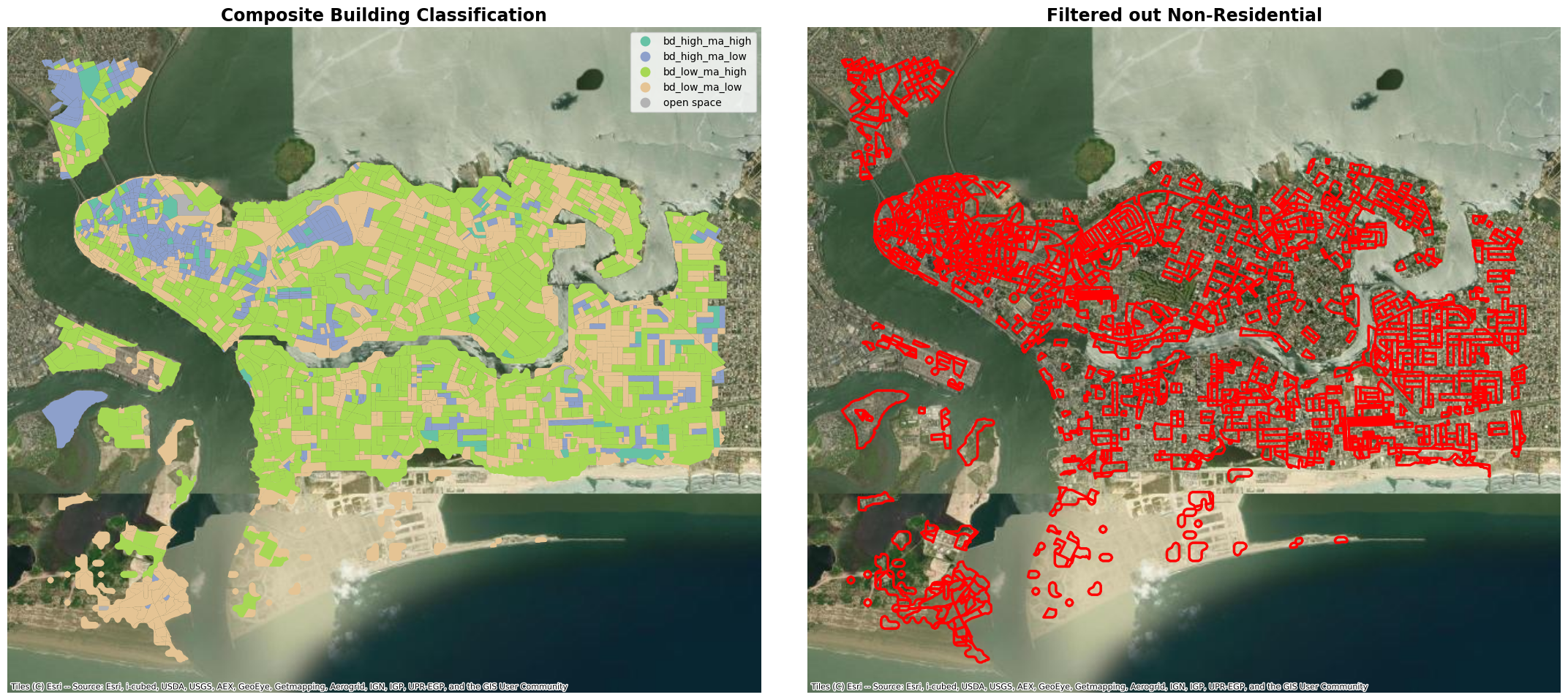

Now that we have filtered out some non-residential areas, we can find the blocks that are likely to have higher populations. building_count_density is the number of buildings / area. This is likely to return low values for blocks dominated by large apartment buildings. Instead we will use building_area_density which is the total building area / block area. We will keep only buildings in the top 75th percentile of this variable.

# Get top 25% of building area percentage
thresh = gdf_res["building_area_percentage"].quantile(0.75)
gdf_dense = gdf_res[
    gdf_res["building_area_percentage"] >= thresh
].copy()

# Create side-by-side plots
fig, axes = plt.subplots(
    1, 2,
    figsize=(22, 10)
)

# Plot building area percentage
gdf.plot(
    column="building_area_percentage",
    ax=axes[0],
    cmap="turbo",
    legend=True,
    legend_kwds={
        "label": "Building Area (%)",
        "shrink": 0.5
    },
    linewidth=0
)

cx.add_basemap(
    axes[0],
    source=cx.providers.Esri.WorldImagery
)

axes[0].set_title(
    "Building Area Percentage",
    fontsize=17,
    fontweight="bold"
)

axes[0].set_axis_off()


# Plot top 25% of building area percentage
gdf_dense.plot(
    ax=axes[1],
    facecolor="none",
    edgecolor="red",
    linewidth=2.5
)

cx.add_basemap(
    axes[1],
    source=cx.providers.Esri.WorldImagery
)

axes[1].set_title(
    "Top 25%: Building Area Percentage",
    fontsize=17,
    fontweight="bold"
)

axes[1].set_axis_off()


# Create layout
plt.subplots_adjust(
    left=0.01,
    right=0.99,
    bottom=0.01,
    top=0.92,
    wspace=0.03
)

plt.show()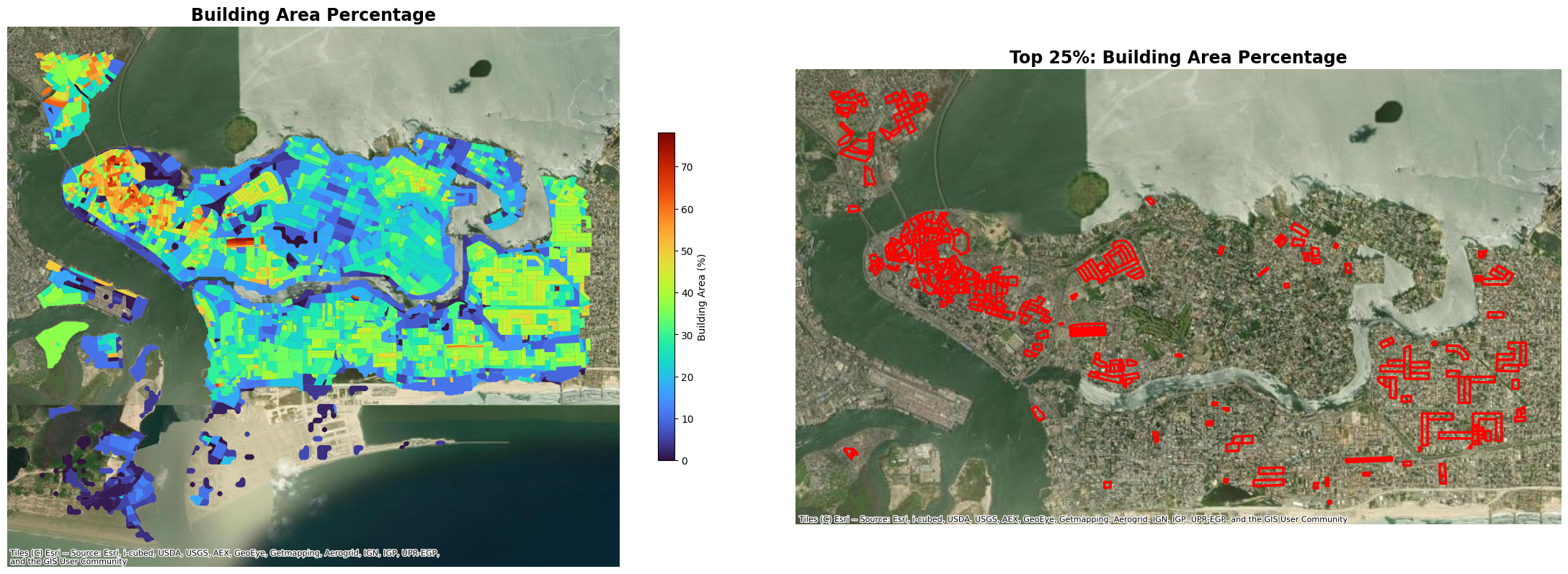

There is one limitation with our previous selection of blocks is while we selected those with the most area covered by buildings, that does not account for vertical space that may be inhabited such as high rise apartment buildings. To improve our selection and capture vertical space, we can multiply the building_area_percentage by the gbuilding_mean_height.

# Get top 25% of building mean height x building area percentage
gdf_res["density_height"] = (
    gdf_res["gbuilding_mean_height"] *
    gdf_res["building_area_percentage"]
)

thresh = gdf_res["density_height"].quantile(0.75)
gdf_dense_height = gdf_res[gdf_res["density_height"] >= thresh].copy()

# Create plot
fig, axes = plt.subplots(
    1, 2,
    figsize=(22, 10)
)

# Plot mean height
gdf.plot(
    column="gbuilding_mean_height",
    ax=axes[0],
    cmap="turbo",
    legend=True,
    legend_kwds={
        "label": "Mean Building Height (m)",
        "shrink": 0.5
    },
    linewidth=0
)

cx.add_basemap(
    axes[0],
    source=cx.providers.Esri.WorldImagery
)

axes[0].set_title(
    "Mean Building Height",
    fontsize=17,
    fontweight="bold"
)

axes[0].set_axis_off()


# Plot blocks in top 25%
gdf_dense_height.plot(
    ax=axes[1],
    facecolor="none",
    edgecolor="red",
    linewidth=2.5
)

cx.add_basemap(
    axes[1],
    source=cx.providers.Esri.WorldImagery
)

axes[1].set_title(
    "Top 25%: Building Height × Building Area",
    fontsize=17,
    fontweight="bold"
)

axes[1].set_axis_off()

# Create layout
plt.subplots_adjust(
    left=0.01,
    right=0.99,
    bottom=0.01,
    top=0.92,
    wspace=0.03
)

plt.show()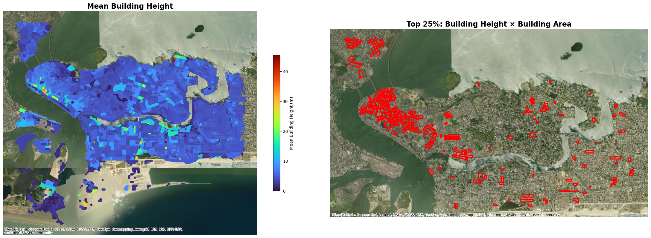

Now that we have narrowed down our blocks to those with the most building space, it is time to target the 20 blocks with the lowest vegetation. For this selection, we have two options: NDVI which is a normalized vegetation index and EVI which is an enhanced vegetation index. Both of the indices work similarly, capture the amount of healthy green vegetation. EVI was designed to work in some environments where NDVI had limitations such as heavy biomass areas like rainforests. Both are widely used measures of greeness, and thus we can compare them both in this setting by selecting the filtered blocks with the lowest NDVI and EVI values.

# Get 10 blocks with lowest NDVI
gdf_sorted = gdf_dense_height.sort_values("ndvi_mean")
gdf_low_ndvi = gdf_sorted.head(20)

# Get 10 blocks with lowest EVI
gdf_sorted = gdf_dense_height.sort_values("evi_mean")
gdf_low_evi = gdf_sorted.head(20)


fig, axes = plt.subplots(1, 2, figsize=(15, 7))


gdf_low_ndvi.plot(
    ax=axes[0],
    facecolor="none",
    edgecolor="red",
    linewidth=2.5
)

cx.add_basemap(
    axes[0],
    source=cx.providers.Esri.WorldImagery
)

axes[0].set_title("20 Blocks with Lowest NDVI", fontsize=16)
axes[0].set_axis_off()


gdf_low_evi.plot(
    ax=axes[1],
    facecolor="none",
    edgecolor="red",
    linewidth=2.5
)

cx.add_basemap(
    axes[1],
    source=cx.providers.Esri.WorldImagery
)

axes[1].set_title("20 Blocks with Lowest EVI", fontsize=16)
axes[1].set_axis_off()

plt.tight_layout()
plt.show()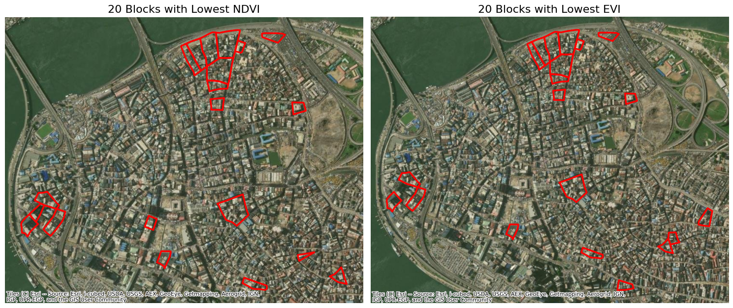

The comparison between NDVI and EVI match pretty closely in this context, with the exception of a couple of blocks which appear in one and not the other. Now lets print out a table with these blocks and their location to identify the target locations for urban greening.

# Get all unique block IDs from both datasets
block_ids = sorted(
    set(gdf_low_ndvi["block_id"]) |
    set(gdf_low_evi["block_id"])
)

# Create comparison table
comparison = pd.DataFrame({"block_id": block_ids})

# Whether block appears in each dataset
comparison["Identified by NDVI"] = comparison["block_id"].isin(
    gdf_low_ndvi["block_id"]
)

comparison["Identified by EVI"] = comparison["block_id"].isin(
    gdf_low_evi["block_id"]
)

# Get geometries from either dataset
geometry_lookup = pd.concat([
    gdf_low_ndvi[["block_id", "geometry"]],
    gdf_low_evi[["block_id", "geometry"]]
]).drop_duplicates("block_id")

# Convert to WGS84 for latitude/longitude
geometry_lookup = geometry_lookup.to_crs(epsg=4326)

# Calculate polygon centroids
geometry_lookup["longitude"] = geometry_lookup.geometry.centroid.x
geometry_lookup["latitude"] = geometry_lookup.geometry.centroid.y

# Add coordinates to comparison table
comparison = comparison.merge(
    geometry_lookup[["block_id", "latitude", "longitude"]],
    on="block_id",
    how="left"
)

comparison

	block_id	Identified by NDVI	Identified by EVI	latitude	longitude
0	blk_75282	False	True	6.452827	3.392308
1	blk_75321	True	True	6.454447	3.390650
2	blk_75335	True	True	6.454796	3.394436
3	blk_75346	False	True	6.455229	3.394763
4	blk_75363	True	True	6.455622	3.386639
5	blk_75440	True	False	6.455711	3.392847
6	blk_75969	True	False	6.457184	3.386050
7	blk_75971	True	True	6.457086	3.380601
8	blk_75999	False	True	6.456229	3.396431
9	blk_76000	True	True	6.457215	3.381782
10	blk_76013	True	True	6.462447	3.389003
11	blk_76045	True	True	6.458188	3.381412
12	blk_76054	True	False	6.457647	3.380988
13	blk_76074	True	True	6.463938	3.389132
14	blk_76081	True	True	6.457761	3.389766
15	blk_76113	True	True	6.464982	3.390013
16	blk_76149	True	True	6.464695	3.388141
17	blk_76167	True	True	6.463271	3.388977
18	blk_76168	True	True	6.464931	3.388687
19	blk_76202	True	True	6.465125	3.389451
20	blk_76220	True	True	6.464418	3.387826
21	blk_76286	True	True	6.462284	3.392613
22	blk_76449	True	True	6.465426	3.391504